A Deep-Learning-Based Particle-in-Cell Method for Plasma Simulations
Xavier Aguilar PDC
Particle-in-cell (PIC) methods are an important group of methods to help us understand the behaviour of plasma dynamics in complex phenomena and systems. Parallel PIC codes, such as VPIC [1], iPIC3D [2], and Warp-X [3], are run on the largest supercomputers in the world, and they are being applied in fields ranging from space physics and astrophysics to accelerators, fusion reactors or laser-plasma devices. However, simulating plasma phenomena is complex and requires a lot of computational power.
Lately, Machine Learning (ML) and Deep Learning (DL) have emerged in high-performance computing (HPC) as a viable methodology to complement classical computational approaches. For example, DL methods are being used in computational fluid dynamics [4], weather forecasting [5], and with DL-based preconditioners and linear solvers [6,7].
This article presents some research work on the use of Deep Learning techniques applied to PIC methods. This work [8] was the result of a collaboration between one of PDC’s application experts, Xavier Aguilar, and Stefano Markidis from the CST Division at KTH, and demonstrates that integrating DL techniques within PIC methods is a promising approach for developing new PIC methods beyond the current ones.
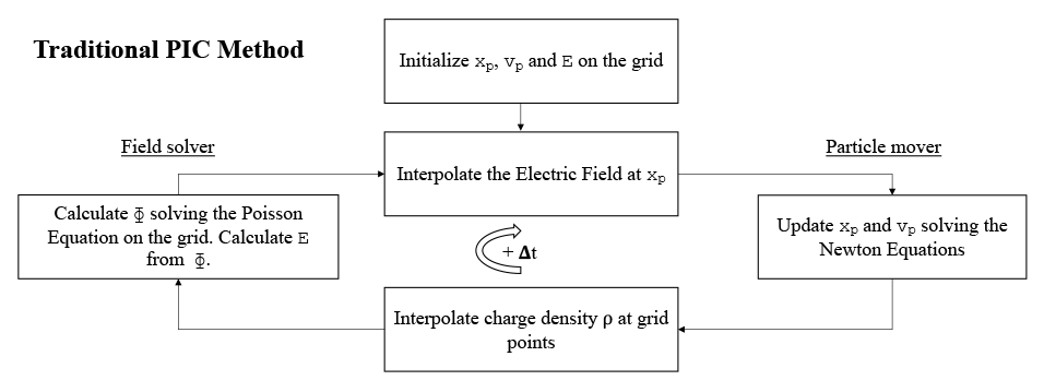
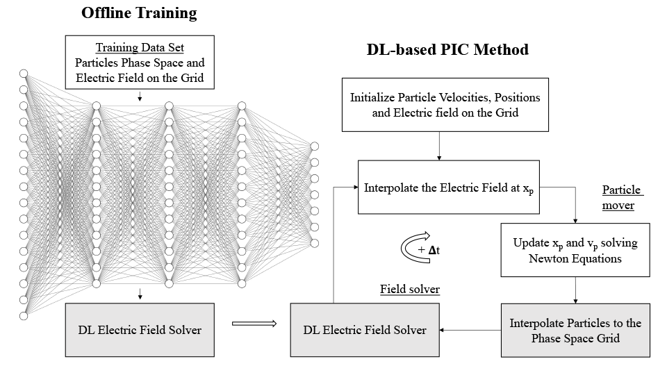
Traditional PIC methods use the algorithm depicted above. They start with an initialization phase, followed by a computational cycle which is repeated hundreds of thousands of times during the simulation. This computational cycle computes the electric and magnetic fields at particle positions, moves particles, computes charge densities on the grid, computes the electrostatic field using Maxwell’s equations, and finally computes the electric field. We took this algorithm and modified it by introducing neural networks in its computational phase. In other words, we substituted some classical computations with DL as depicted in the figure below (in the grey boxes). The new DL-based PIC algorithm still retains the interpolation step to compute the electric field at the particle positions, as well as the particle mover, but uses an electric field solver that is the result of DL neural network training.
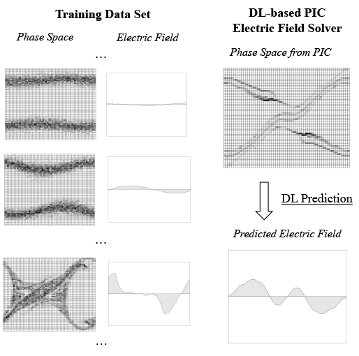
To train the neural network, we produced a data set of images representing a discretized particle phase-space together with its associated electric field for the two-stream instability, which is a well-known plasma benchmark. The figure below shows examples of several phase-space grids together with their electric fields. We generated thousands of these pairs using classical simulations and used them to teach a neural network to predict the electric field from a phase-space grid. More concretely, we generated 40,000 phase-space grids and 40,000 electric fields from classical simulations using different initial parameter configurations, that is, initial beam velocity and thermal speed. The total size of our initial data set was 5.2GB. We used this data to train two different network architectures, a Multilayer Perceptron (MLP) and a Convolution Neural Network (CNN). We ran our experiments on two 12-core Intel E5-2690V3 Haswell processors connected to an NVIDIA Tesla K80 GPU. For more details on the experiments and the setup, refer to the original paper [8].
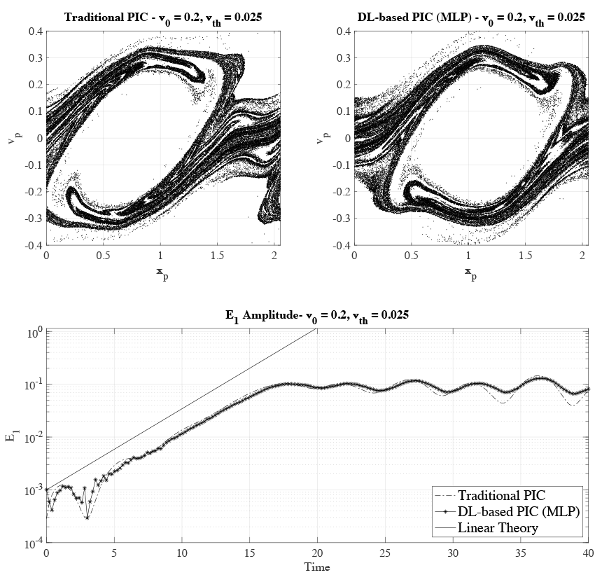
Our initial experiments showed that the MLP had a better mean absolute error on the test data, and it was also much faster to train, and therefore, we decided to focus our efforts on the DL-solver using the MLP. First, we validated the results of the DL-based PIC method using a configuration that was not included in the initial data set. The top panel of the figure below shows the phase-space grid for the classical simulation and the DL approach. The x-axis represents space, and the y-axis is particle velocity. The phase-space plots are not exactly equal because the beam instability starts at different points in time in the two simulations. However, they show similar qualities – for example, how particles are distributed and the size of the phase-space hole – thereby indicating that both simulations produce similar results. Moreover, we validated the results of the DL-based PIC against the results of analytical theory, which provided us with the growth rate of the more unstable mode in the two-stream instability in the cold-beam v0 >> vth approximation. The bottom panel in the figure shows the electric field amplitude for the most unstable mode E1 during the two-stream instability simulation. The solid line is the slope predicted by the linear theory, and the other two are the traditional PIC and the DL-based PIC, respectively. The plot shows how, during the linear phase of the instability (the first phase of the simulation when E1 grows exponentially), both simulations follow the slope predicted by the linear theory, thus validating our results.
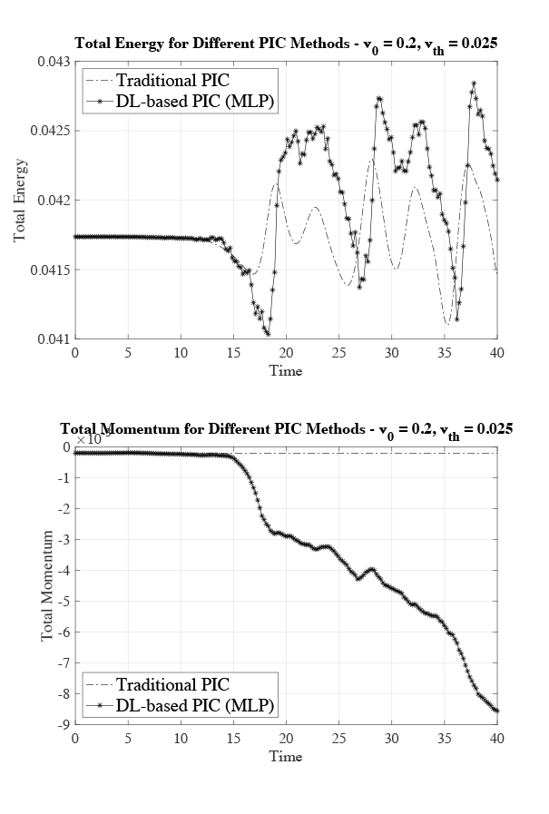
We also monitored how precisely the total energy and momentum were conserved in our simulations. The top graph in the figure below shows the total energy for the classical PIC and the DL-based PIC. Both methods conserve the total energy with a maximum variation of approximately 2%, and therefore we can say that they have similar behaviour when it comes to energy conservation. The lower plot in the figure below shows the evolution of the total momentum during the simulation. In this case, the traditional PIC conserves the momentum, whereas the DL-based approach does not conserve it.
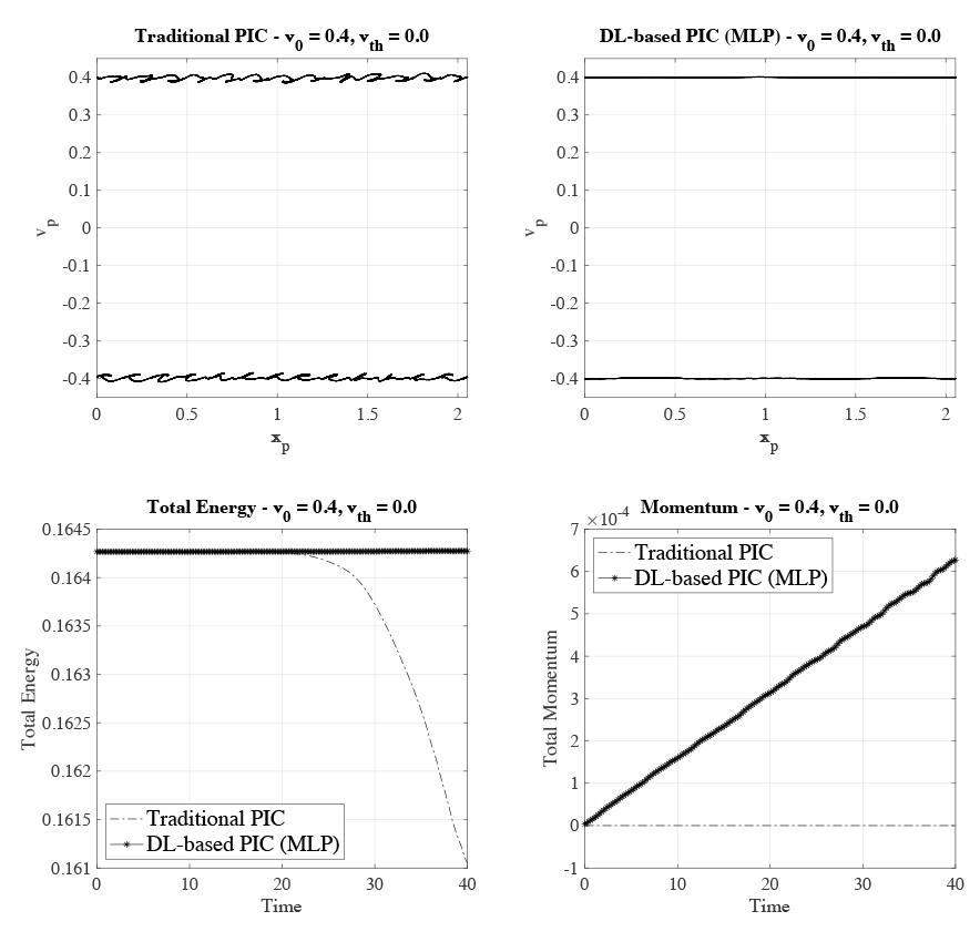
As a final experiment, we simulated a system that is stable against the two-stream instability where the two beams should continue to stream. The top panel of the figure below shows the phase space for both versions at timestep 40. It can be noticed that the classical PIC exhibits a non-physical behaviour, visible in ripples pictured in the phase space. This is called cold-beam instability, and it is a well-known numerical instability that affects momentum and energy conservation in PIC methods. As can be seen in the figure, the DL-based approach is not affected by this cold-beam instability. This numerical instability can also be seen in the total energy conservation of the traditional PIC (left-hand picture in the lower panel of the figure below). While the numeral instability is not present in the DL-based PIC, it still does not conserve the momentum, as can be seen in the right-hand plot in the lower panel of the figure below.
As we have seen in this article, Deep Learning is a promising field that can open new paths to develop novel PIC methodologies. We have demonstrated that our new DL-approach produces correct results, and it is stable against the cold-beam instability. However, these are just the first steps towards the integration of DL techniques into PIC methods. More studies such as spectral error analysis of the electrical field values are needed in order to have a better understanding of such DL-based PIC methods. Furthermore, the use of other networks architectures should be explored. For example, using ResNets or Physics-Informed Neural Networks (PINN) would allow us to include energy and conservation law equations into the network itself, thereby increasing the physical accuracy of the system. Future work would also include characterising the performance of this new DL approach, as well as extending the model to 2D and 3D systems.
References
- K. J. Bowers, B. J. Albright, L. Yin, W. Daughton, V. Roytershteyn, B. Bergen, and T. Kwan, “Advances in petascale kinetic plasma simulation with vpic and roadrunner,” in Journal of Physics: Conference Series, vol. 180, no. 1. IOP Publishing, 2009, p. 012055.
- S. Markidis, G. Lapenta, and R. Uddin, “Multi-scale simulations of plasma with iPIC3D,” Mathematics and Computers in Simulation, vol. 80, no. 7, pp. 1509–1519, 2010.
- J.-L. Vay, A. Almgren, J. Bell, L. Ge, D. Grote, M. Hogan, O. Kononenko, R. Lehe, A. Myers, C. Ng et al., “Warp-x: A new exascale computing platform for beam–plasma simulations,” Nuclear Instruments and Methods in Physics Research Section A: Accelerators, Spectrometers, Detectors and Associated Equipment, vol. 909, pp. 476–479, 2018.
- X. Guo, W. Li, and F. Iorio, “Convolutional neural networks for steady flow approximation,” in Proceedings of the 22nd ACM SIGKDD international conference on knowledge discovery and data mining, 2016, pp. 481–490.
- R. Pradhan, R. S. Aygun, M. Maskey, R. Ramachandran, and D. J. Cecil, “Tropical cyclone intensity estimation using a deep convolutional neural network,” IEEE Transactions on Image Processing, vol. 27, no. 2, pp. 692–702, 2017.
- S. Markidis, (2021). The old and the new: Can physics-informed deep-learning replace traditional linear solvers?, Frontiers in Big Data, 92.
- T. Ichimura, K. Fujita, M. Hori, L. Maddegedara, N. Ueda, and Y. Kikuchi, “A fast scalable iterative implicit solver with Green’s function-based neural networks,” in 2020 IEEE/ACM 11th Workshop on Latest Advances in Scalable Algorithms for Large-Scale Systems (ScalA). IEEE, 2020, pp. 61–68.
- X. Aguilar and S. Markidis, “A Deep Learning-Based Particle-in-Cell Method for Plasma Simulations,” 2021 IEEE International Conference on Cluster Computing (CLUSTER), 2021, pp. 692-697, doi: 10.1109/Cluster48925.2021.00103.