Tracking Large Data Sets
Miguel Zavala-Aké, Niclas Jansson, Mohamad Rezaei, Marco Atzori & Philipp Schlatter, KTH, & Erwin Laure, Max Planck Computing and Data Facility
Introduction
Handling massive amounts of data is a vital issue in the Exascale age. In some areas, such as N-body cosmology, meteorology, Monte Carlo simulations or ocean eddy analysis, this issue is addressed by processing the data at the same time as it is generated. PDC is involved in the quest to overcome the difficulties associated with dealing with huge sets of data as part of its role in the European Centre of Excellence for Engineering Applications (EXCELLERAT) project.
In a majority of engineering and scientific applications, real-time processing aims to prepare data for visualization. (Visualization means converting the data into graphical representations, such as images, maps or charts, that make it easier to see patterns or trends in the data). However, reducing the volume of the data – by means of compression or feature extraction – is also important. Compressing the data is appropriate when a combination of post hoc and in situ processing is used: post hoc processing means the data is processed after it is produced, while in situ means the data is processed while it is being created. If the data-processing strategy is known in advance, in situ feature extraction is a more appropriate approach.
PDC's efforts have been focused on the challenges related to data reduction via the real-time handling of algorithms already available in the Visualization Toolkit (VTK) software. This data handling is performed at PDC using a high-performance computing (HPC) analysis tool, known as PAAKAT (which means “looking at” in the Mayan language).
An HPC In Situ Visualization Tool
The PAAKAT library has been designed as an HPC tool which encourages scalability and portability of in situ analysis in large-scale simulations. The emphasis is on reducing the output data of such simulations during run-time by using algorithms already available in VTK. The main difference regarding the great deal of effort made to develop software specializing in the solution of in situ visualization and analysis is related to the fact that PAAKAT encourages scalability and portability. This has been done by focusing on data arising from VTK filters while it obviates the need for rendering in the Paraview source code (version 5.6). These modifications encourage the use of the C++ VTK API, so that the need for third-party software components is reduced. As a consequence of these modifications, filters must be implemented using C++ instead of the Python scripts created by ParaView.
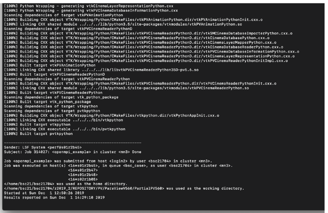
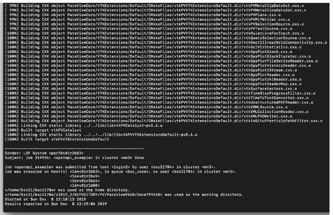
The figures above show the compilation times for two different ParaView setups. The first case corresponds to ParaView 5.6 with Python where renderings are considered but without the graphical user interface. In the second case, the modified ParaView is compiled. While in the first case the compilation time was about 99 minutes, in the second case it only took around 9 minutes. In both cases, 64 cores were used. As future work, more computer systems and compilers must be tried to investigate reductions in compilation time.
A Parallel Time Tracking Algorithm
This section briefly describes an example which uses the modified version of ParaView. This example features a parallel tracking algorithm which has been implemented exclusively using the C++ VTK API. The goal is to analyze the time evolution of coherent structures in a given turbulent flow. The algorithm is divided into three main parts (see below). Firstly, a scalar function f(r,t) = c0 defines a set of points (isosurfaces) which take on a constant value c0. Then, all these points are grouped in subsets (clusters), each of them characterized by a unique number. Finally, a search for overlappings between subsets belonging to different time steps is performed. Subsets are considered to be connected if overlappings between them exist. The search for overlappings is repeated each time step, so that the connections that are found make it possible to track the time for each cluster. The following subsections give details for each of these.
Isosurfaces and Clustering
Given a scalar field defined by a function, f(r,t), isosurfaces and clusters are obtained using algorithms that can be found in the Visualization Toolkit library. Thresholding is performed by a recursive algorithm which allows users to identify a portion of an isosurface (cluster) through a unique number. Then these sets of numbers can be used to separate, and carefully investigate, each cluster.
Temporal Connectivities
In order to track each cluster over time, connectivities between clusters allocated in different time steps must be established. Here these connectivities are established in three steps. Firstly, each cluster is confined within the smallest box (aligned to the Cartesian coordinate system) which can hold all its points. Then, a search for overlappings is performed between a bounding box belonging to the current time step and bounding boxes held in a previous time step. Finally, if two bounding boxes (allocated in different time steps) overlap, then a Boolean operation is performed between the clusters contained by each bounding box. A positive result from the Boolean intersection of these clusters means that overlappings between these clusters exist. Such an overlapping can be understood as indicating that a temporal connection exists between those two clusters.
Overlapping
In the simplest cases, a cluster allocated in a given time could be either completely unconnected to any other clusters or connected with only one previous cluster. In the first case, it is possible to assume that a new cluster has emerged, while in the second case, the tracked cluster has only suffered small changes. In more complicated cases, multiple connectivities indicate that the current cluster results from the merging of multiple clusters. Other possible kinds of connections (merging and splitting) are depicted in the figure below.
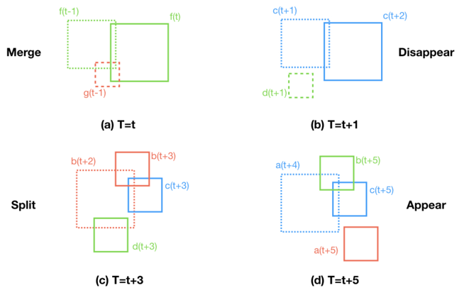
Merging connectivities take place when, in a given time, two or more previous clusters overlap a single cluster, so that some of the previous clusters seem to have disappeared. Now, these merges could be either total or partial. A total merge occurs when each of the previous clusters is connected to each of the current clusters. A partial merge takes place when at least one previous cluster does not overlap any current cluster. This means that some of the previous clusters are temporally unconnected. In this situation, it could be considered that the unconnected clusters were either embedded (by a contiguous cluster) or vanished (perhaps due to the nature of the physics of the underlying problem). Finally, it is worth noting that, when merges take place, the total number of current clusters is lower than the number in the previous time step.
Unlike merging, splitting connectivities takes place when a single previous bounding box overlaps two or more current bounding boxes. In these cases, new clusters seem to have emerged, so that the total number of current clusters is larger than in the previous step. Total splitting occurs when each cluster that emerges is connected with some of the previous clusters. In contrast, when partial splitting occurs, any unconnected clusters that arise are supposed to be entirely new.
The set of temporal connectivities established at each time step can be used to compose a graph which shows how the interaction between clusters evolves over time. In the next section, this is discussed in depth.
Time Tracking Graph
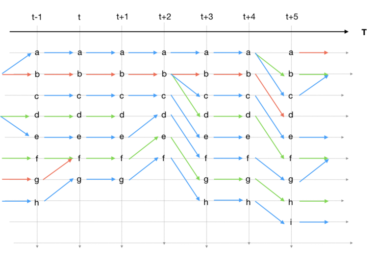
Merging and splitting of clusters could happen at any time and anywhere. A time tracking graph (as shown in the figure below) helps us to take an in-detail look at when merging and splitting take place. In these graphs, the set of cluster identifiers are represented as vertices while edges indicate the temporal connectivities resulting from searching for overlappings (see the previous section). Vertices are grouped according to the time step (or stages) to which they belong and, in turn, these time steps are organized in chronological order. In this way, edges can only traverse from one time step to another.
In the figure below, temporal connectivities shown in the figure above are used to depict a time tracking graph. Cluster identifiers are placed from top to bottom, while time flows from left to right. Lowercase letters are used to identify each vertex, while arrows are used for edges. In each stage, arrows indicate input and output connections. An input connection relates a previous time step with the current stage, while an output connection relates the current stage with the next time step. Now, the four stages (t, t+1, t+3, and t+5) shown in the figure above can be found here. At stage t, seven clusters exist, along with eight input connections and seven output connections. Each cluster is simply connected, with the exception of cluster f, which has two input connections (ft−1 → ft and gt−1 → ft) that arise from the merging of clusters f and g at time step t−1. Finally, it is worth noting that, due to the merging, in this stage the number of clusters has decreased with respect to the previous time step. As a consequence, the last cluster at t−1 has been renamed. This means that, from the search for overlappings, cluster ht−1 and gt are simply connected, in other words, these two clusters are the same. The previous procedure can be repeated for the rest of the stages. At t+1, the number of clusters remains unchanged. For the next stage, the number of clusters has decreased, due to the fact that cluster dt+1 has died out.
Results
In the next case study, the goal is to analyze the time evolution of coherent structures in a turbulent flow. The numerical simulation makes use of 2×10⁶ elements, 1×10² time steps, 256 MPI processes, and the parallel code Nek5000 to solve a direct numerical simulation (DNS) of a turbulent flow at a friction Reynolds number Reτ = 180.
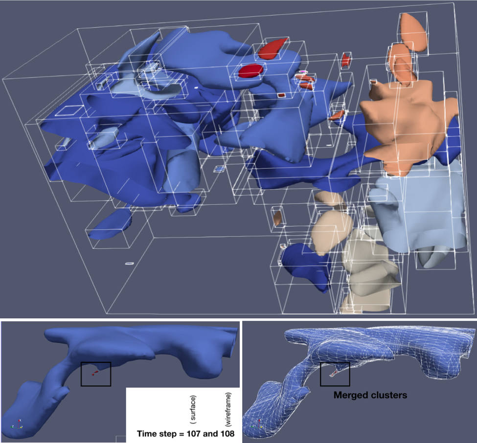
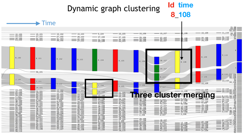
The figure below shows a set of clusters (coherent structures) at time step 107, along with three extracted clusters (8, 58 and 59) and their evolution towards a simple cluster (8 at time step 108). Their evolution over ten time steps (dynamic graph clustering) and the corresponding chronology in which the parallel workflow of the tracking algorithm is executed (parallel activity trace) are shown in the lower two images respectively.
The time tracking graph related to this case is plotted by using a Sankey diagram in which temporal connectivities between clusters allocated in different time steps can be represented. In the figure below, time flows from left to right, clusters are represented as vertices (coloured rectangles) with temporal connectivities (thick gray lines) as edges between them. Each vertex is labelled as id_time, which corresponds to its cluster identifier id (as given by vtkConnectivityFilter) and the current time step time. Thus, the merging of clusters shown in the figure above is represented in the graph as three vertices (8_107, 58_107 and 59_107) connected with a simple one (8_108) through three edges. Taking as a reference time t=107, it is possible to see that these clusters arise from the splitting of cluster 8 at time t=106. In the same way, the evolution of each and every one of the clusters can be followed over the simulation time.
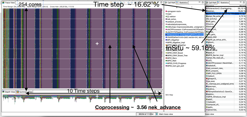
The parallel activity trace shown in the figure below gives a first performance analysis of the tracking algorithm. In the trace that is shown, 256 MPI processes are used to execute ten time steps, which correspond to steps from 100 to 109. For these steps, the statistics view shows that the execution time of the in situ analysis (vtkCPVTKPipeline :: CoProcess ~ 59.10%) is 3.56 times bigger than for the Nek5000 solver (esolver ~ 16.62%).
Conclusions
As part of the EXCELLERAT project, an in situ instrumentation for the code Nek5000 has been prepared and used to perform the time evolution analysis of coherent structures. For this instrumentation, the HPC in situ analysis tool PAAKAT has been used. The performance analysis shows a low increase in the total execution time (which includes simulation and analysis times). In addition, it should be considered that in post hoc processing the simulation program needs to stop and wait for the application of some data reduction method, which increases the total execution time. The ongoing work considers efficiency and scalability tests in different exascale machines.